
Pie Chart Perfection: A Beginner’s Guide
Welcome to the wonderful world of pie charts in Google Sheets! If you’re new to the concept of data visualization or just looking to up your chart game, you’ve come to the right place. In this beginner’s guide, we’ll show you how to create the perfect pie chart that will not only impress your colleagues but also effectively communicate your data in a visually appealing way.
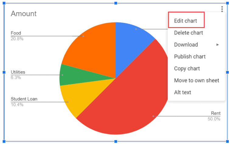
Image Source: productivityspot.com
Pie charts are a great tool for showcasing proportions and percentages within a dataset. They allow you to easily see the distribution of categories or values at a glance, making it a popular choice for businesses, educators, and researchers alike. With Google Sheets, creating a pie chart is a breeze, and with a few simple steps, you’ll be well on your way to pie chart perfection.
To begin, make sure you have your data ready in Google Sheets. Whether it’s sales figures, survey responses, or any other type of numerical data, organizing your information in a clear and concise manner is key to creating an effective pie chart. Once you have your data set up, select the range of cells you want to include in your chart.
Image Source: golayer.io
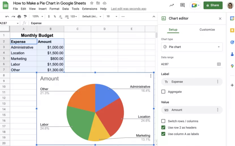
Next, navigate to the Insert menu at the top of the Google Sheets interface and select Chart. This will open up the chart editor where you can choose the type of chart you want to create. In this case, we’re focusing on pie charts, so make sure to select Pie chart from the list of chart types.
Now that you’ve selected your chart type, it’s time to customize your pie chart to make it truly shine. You can adjust the colors, labels, and other visual elements to make your chart pop and ensure it effectively communicates your data. Experiment with different options until you find the perfect combination that suits your needs.
One important thing to keep in mind when creating a pie chart is to avoid overcrowding it with too many categories. While it can be tempting to include every piece of data you have, a cluttered pie chart can be confusing and difficult to interpret. Stick to a manageable number of categories to keep your chart clear and easy to read.
Another tip for pie chart perfection is to use labels and legends to provide context and help viewers understand the information being presented. Labels can be added to each slice of the pie to show the exact percentage or value it represents, while legends can provide additional information about each category.
Once you’re satisfied with your pie chart design, it’s time to insert it into your Google Sheets document. Simply click Insert in the chart editor and choose whether you want to insert the chart as a new sheet or as an image in your current sheet. Your pie chart will now be displayed for all to see, showcasing your data in a visually appealing and easy-to-understand manner.
In conclusion, creating a pie chart in Google Sheets is a fun and simple way to bring your data to life and make it more engaging for your audience. By following the steps outlined in this beginner’s guide, you’ll be well on your way to mastering the art of pie chart perfection. So go ahead, slice and dice your data like a pro, and watch as your numbers transform into delicious visuals that will impress and inform anyone who sees them. Happy charting!
Slicing and Dicing Data Like a Pro
Are you ready to take your data visualization skills to the next level? In the world of creating pie charts in Google Sheets, mastering the art of slicing and dicing your data like a pro is essential. With a few simple tricks and tips, you’ll be able to transform your raw numbers into delicious visuals that tell a compelling story.
One of the first steps in creating a pie chart is to carefully select the data that you want to represent. This is where slicing and dicing comes into play. By breaking down your data into smaller, more manageable pieces, you’ll be able to create a pie chart that is both visually appealing and informative. Whether you’re working with sales figures, survey responses, or any other type of data, the key is to identify the most relevant and important information that you want to convey.
Once you have your data sliced and diced, it’s time to start creating your pie chart in Google Sheets. The beauty of using Google Sheets for data visualization is that it offers a wide range of tools and features to help you customize your chart to your liking. From changing the colors and labels to adjusting the size and layout, the possibilities are endless.
One of the best ways to slice and dice your data like a pro is to use the pivot table feature in Google Sheets. This tool allows you to quickly summarize and manipulate your data in a way that makes it easier to create a pie chart. By organizing your data into categories and subcategories, you’ll be able to see patterns and trends that may not have been immediately obvious.
Another helpful tip for slicing and dicing your data is to use filters and sort functions in Google Sheets. These tools allow you to quickly and easily rearrange your data in a way that makes it easier to create a pie chart. Whether you’re looking to focus on specific data points or highlight certain trends, filters and sort functions can help you make sense of your data in a visual way.
In addition to slicing and dicing your data, it’s also important to consider the design and layout of your pie chart. While Google Sheets offers a variety of customization options, it’s important to keep in mind the principles of good design. Make sure that your chart is easy to read and understand, with clear labels and colors that make it visually appealing.
When it comes to creating a pie chart in Google Sheets, mastering the art of slicing and dicing your data like a pro is key. By carefully selecting and organizing your data, using tools like pivot tables, filters, and sort functions, and paying attention to design and layout, you’ll be able to create a pie chart that tells a compelling story. So go ahead, slice and dice your data with confidence, and watch as your numbers come to life in a delicious visual display.
Turning Numbers into Delicious Visuals
Slice and Dice: Mastering the Art of Creating a Pie Chart in Google Sheets
Turning Numbers into Delicious Visuals
When it comes to data visualization, pie charts are a classic choice for displaying numerical information in an easy-to-understand format. With Google Sheets, turning your numbers into delicious visuals has never been easier. In this article, we will explore the art of creating a pie chart in Google Sheets and how you can master the process to make your data come to life.
Before we dive into the steps of creating a pie chart, let’s first understand the importance of visualizing data. Numbers and statistics can often be overwhelming or difficult to comprehend at first glance. By transforming these numbers into visual representations like pie charts, you can make your data more engaging and easier to interpret.
Google Sheets offers a user-friendly platform for creating pie charts, allowing you to customize your visuals and present your data in a visually appealing way. Whether you are a beginner or an experienced data analyst, mastering the art of creating pie charts in Google Sheets can elevate your data presentation skills.
Now, let’s get started on turning your numbers into delicious visuals with Google Sheets:
Step 1: Organize Your Data
Before creating a pie chart, it is essential to organize your data in Google Sheets. Make sure your data is clear, concise, and relevant to the information you want to visualize. You can use columns and rows to input your data and ensure that it is accurate and up-to-date.
Step 2: Select Your Data
Once your data is organized, select the cells that you want to include in your pie chart. Google Sheets allows you to easily highlight the data you want to visualize, making it simple to turn your numbers into visuals.
Step 3: Insert a Pie Chart
After selecting your data, go to the Insert tab in Google Sheets and choose the option for Chart. From the chart options, select Pie chart to create a visual representation of your data. Google Sheets offers various customization options for pie charts, allowing you to adjust colors, labels, and other visual elements to suit your preferences.
Step 4: Customize Your Pie Chart
Once you have inserted a pie chart, you can customize it to enhance its visual appeal. Google Sheets provides options for adjusting the chart title, labels, legend, and other design elements to make your pie chart visually engaging and informative. Experiment with different customization options to create a pie chart that effectively communicates your data.
Step 5: Analyze and Interpret Your Chart
After creating and customizing your pie chart, take the time to analyze and interpret the visual representation of your data. Pie charts allow you to easily compare different categories or data points, making it simpler to identify trends, patterns, and relationships within your data. Use your pie chart to draw insights and conclusions from your data visualization.
By following these steps and mastering the art of creating a pie chart in Google Sheets, you can turn your numbers into delicious visuals that effectively communicate your data. Whether you are presenting data for a business report, a school project, or personal analysis, pie charts can help you make your data more engaging and understandable.
So, the next time you have numerical information that you want to showcase, consider creating a pie chart in Google Sheets. With a few simple steps and some creativity, you can transform your numbers into delicious visuals that captivate your audience and make your data come to life.
Google Sheets Pie Charts Made Easy
Are you ready to slice and dice your data like a pro? Look no further than Google Sheets, where creating beautiful pie charts is a breeze. With just a few simple steps, you can turn your boring data into a delicious visual feast that will not only impress your colleagues but also help you better understand your data.
Pie charts are a great way to showcase the proportion of different categories within a dataset. Whether you’re analyzing sales data, survey results, or any other type of information, a pie chart can help you quickly identify trends and patterns. And with Google Sheets, creating a pie chart is easier than ever.
To get started, all you need is a Google Sheets account and a dataset that you want to visualize. Simply input your data into a spreadsheet, making sure to assign each category a corresponding value. Once your data is ready, here’s how you can create a beautiful pie chart in Google Sheets:
1. Select the data you want to include in the pie chart. This can be a single column or row of data, or multiple columns or rows. Simply click and drag to highlight the cells that contain your data.
2. Click on the Insert menu at the top of the Google Sheets interface, then select Chart from the dropdown menu. This will open the Chart Editor on the right side of the screen.
3. In the Chart Editor, click on the Chart type dropdown menu and select Pie chart. You can also customize the appearance of your chart by changing the colors, labels, and other settings.
4. Once you’re happy with how your chart looks, click on the Insert button in the Chart Editor to add the pie chart to your spreadsheet. You can then resize and move the chart to wherever you want it to appear.
And that’s it! With just a few clicks, you’ve transformed your boring data into a beautiful pie chart that is both visually appealing and informative. But the fun doesn’t stop there – Google Sheets offers a variety of customization options that allow you to further enhance your pie chart and make it truly stand out.
For example, you can add a title and labels to your chart to provide additional context and make it easier to understand. You can also adjust the colors and formatting to match your personal style or the branding of your organization. And if you want to dive deeper into your data, you can use the Chart Editor to explore different chart types, add trendlines, and more.
But perhaps the best part of creating a pie chart in Google Sheets is the ability to easily update it as your data changes. If you make any edits to your dataset, your pie chart will automatically reflect those changes, saving you time and ensuring that your visualizations are always up to date.
So why settle for boring, static data when you can turn it into a dynamic, eye-catching pie chart with Google Sheets? Whether you’re a beginner looking to dip your toes into the world of data visualization or a seasoned pro in search of a new tool to add to your arsenal, Google Sheets has everything you need to create stunning pie charts with ease. Happy charting!
how to create a pie chart in google sheets


