Pie Chart Magic: Unleashing Your Inner Data Wizard

Have you ever felt overwhelmed by the sheer amount of data you have to analyze and present in a clear and concise way? Well, fear not! With the power of pie charts in Google Spreadsheet, you can unleash your inner data wizard and create stunning visual representations of your data in just a few simple steps.

Pie charts are a great way to visually represent data and make it easier for your audience to understand the information you are trying to convey. Whether you are presenting sales figures, survey results, or any other type of data, pie charts can help you slice and dice your data into easily digestible pieces.

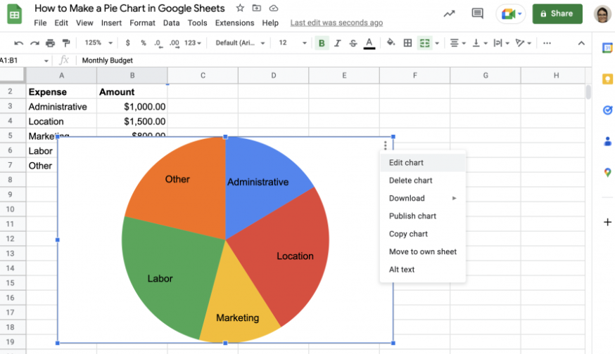
To create a pie chart in Google Spreadsheet, all you need to do is select the data you want to include in your chart, click on the Insert menu, and then choose Chart. From there, you can select the type of chart you want to create (in this case, a pie chart) and customize it to fit your needs.

One of the great things about pie charts in Google Spreadsheet is that you can easily customize them to fit your specific needs. You can change the colors, labels, and even the size of the slices to create a chart that is not only visually appealing but also informative.

Pie charts are also a great tool for comparing different data sets and identifying trends or patterns in your data. By creating multiple pie charts and placing them side by side, you can easily see how different data sets compare to each other and identify any outliers or anomalies.

In addition to being a powerful data visualization tool, pie charts are also a fun and creative way to present your data. You can experiment with different colors, labels, and styles to create a chart that is not only informative but also visually appealing.

So, whether you are a data wizard or just getting started with data analysis, pie charts in Google Spreadsheet are a great tool to have in your arsenal. With just a few simple clicks, you can create stunning visual representations of your data that will impress your audience and help you make sense of your data in a whole new way.

So what are you waiting for? Unleash your inner data wizard and start creating pie charts in Google Spreadsheet today!

Slicing Through Numbers: Google Spreadsheet Tricks

Slice and Dice: Mastering the Art of Creating a Pie Chart in Google Spreadsheet

Slicing Through Numbers: Google Spreadsheet Tricks

Are you ready to slice through numbers and create stunning pie charts in Google Spreadsheet? If so, you’ve come to the right place! In this article, we will explore some tricks and tips to help you master the art of creating pie charts with ease.

Google Spreadsheet is a powerful tool that allows you to organize, analyze, and visualize data in a user-friendly way. One of the most popular ways to visualize data in Google Spreadsheet is through pie charts. Pie charts are excellent for showing proportions and percentages in a clear and visually appealing manner.

So, let’s dive into some Google Spreadsheet tricks that will help you create beautiful pie charts in no time!

Tip 1: Organize Your Data

The first step in creating a pie chart in Google Spreadsheet is to organize your data properly. Make sure that your data is in a clear and structured format, with each category or slice of the pie chart clearly labeled. This will make it easier to create your pie chart and ensure that it accurately reflects the data you are trying to visualize.

Use columns and rows to separate your data, and be sure to include headers for each category. This will help you easily select the data you want to include in your pie chart and make the process smoother and more efficient.

Tip 2: Select Your Data

Once you have organized your data, the next step is to select the data you want to include in your pie chart. To do this, simply click and drag your mouse over the cells containing the data you want to visualize. You can also use the Ctrl key to select multiple non-adjacent cells.

Make sure to include both the category labels and the corresponding data values in your selection. This will ensure that your pie chart accurately represents the proportions of each category.

Tip 3: Insert Your Pie Chart

With your data selected, it’s time to insert your pie chart. In Google Spreadsheet, this can be done with just a few clicks. Simply go to the Insert menu at the top of the screen, hover over Chart, and select Pie Chart from the dropdown menu.

A pie chart will automatically be generated based on the data you selected. You can customize the appearance of your pie chart by changing the colors, labels, and other settings to make it visually appealing and easy to understand.

Tip 4: Customize Your Pie Chart

Once your pie chart is inserted, you can customize it to better suit your needs. You can change the colors of the slices, add a title and labels, adjust the size and style of the chart, and more.

Customizing your pie chart will not only make it look more professional, but it will also help convey your message more effectively. Experiment with different settings until you find the perfect look for your pie chart.

Tip 5: Share and Collaborate

Finally, once you have created your perfect pie chart, it’s time to share it with others. Google Spreadsheet makes it easy to share your charts with collaborators or embed them in presentations or reports.

Simply click on the Share button in the top right corner of the screen, choose who you want to share your chart with, and select the sharing options that best suit your needs. You can also export your chart as an image or PDF to include in other documents.

With these Google Spreadsheet tricks, you can slice through numbers and create stunning pie charts with ease. Whether you’re analyzing sales data, tracking expenses, or visualizing survey results, pie charts are a powerful tool that can help you communicate your message effectively. So, get slicing and start creating beautiful pie charts today!

Slice and Dice: Mastering the Art of Creating a Pie Chart in Google Spreadsheet

Mastering the Art of Pie Charts in 5 Easy Steps

When it comes to visualizing data, pie charts are a classic choice. They are not only visually appealing but also make it easy to understand complex data at a glance. In this article, we will walk you through 5 easy steps to mastering the art of creating a pie chart in Google Spreadsheet.

Step 1: Gather Your Data

The first step in creating a pie chart is to gather the data that you want to visualize. Make sure that your data is organized in a clear and concise manner. For example, if you want to create a pie chart showing the distribution of sales by product category, your data should include the sales numbers for each category.

Step 2: Select Your Data

Once you have gathered your data, select the cells that you want to include in your pie chart. You can do this by clicking and dragging your mouse over the cells or by holding down the Shift key and using the arrow keys to select multiple cells at once.

Step 3: Insert Your Chart

With your data selected, go to the Insert menu in Google Spreadsheet and choose Chart. This will open a sidebar where you can customize your chart. Select Pie chart from the list of chart types and click Insert to add the chart to your spreadsheet.

Step 4: Customize Your Chart

Once your chart is inserted, you can customize it to better reflect your data. You can change the colors of the slices, add a title, and even adjust the size of the chart. Experiment with different options until you find a design that works best for your data.

Step 5: Share Your Chart

Finally, once you have created the perfect pie chart, it’s time to share it with others. You can easily share your chart by clicking on the Share button in Google Spreadsheet and choosing whether to share it with specific people or make it public. You can also embed your chart in a presentation or webpage by using the Publish option.

And there you have it – 5 easy steps to mastering the art of creating a pie chart in Google Spreadsheet. With a little practice and creativity, you can turn your data into stunning visualizations that will impress your colleagues and clients. So why wait? Start creating your own pie charts today and unleash your inner data wizard!

Let’s Get Baking: Creating Stunning Pie Charts!

Pie charts are a delicious way to visually represent data in Google Spreadsheet. Just like baking a pie, creating a pie chart requires the right ingredients and a dash of creativity. In this article, we will explore the art of creating stunning pie charts in Google Spreadsheet.

First things first, gather your data like you would gather ingredients for a pie. Make sure your data is organized and ready to be sliced and diced in your spreadsheet. Once you have your data ready, select the cells that you want to include in your pie chart.

Now, it’s time to start baking your pie chart. In Google Spreadsheet, go to the Insert tab and select Chart. Choose the type of chart you want to create, in this case, a pie chart. Google Spreadsheet will automatically generate a pie chart based on your selected data.

But wait, don’t stop there! Let’s add a little flair to your pie chart. You can customize the colors, labels, and layout of your pie chart to make it truly stunning. Play around with different color schemes and fonts to make your pie chart visually appealing.

Once you are satisfied with the look of your pie chart, it’s time to give it a title. A good title will help the viewer understand what the pie chart is representing. Make sure your title is clear and concise.

Now that your pie chart is ready, it’s time to share it with others. You can easily embed your pie chart in a presentation, report, or email. Simply copy and paste the chart into your desired document.

But creating stunning pie charts doesn’t end there. You can also animate your pie chart to make it more dynamic and engaging. In Google Spreadsheet, go to the Chart menu and select Advanced Edit. Here, you can add animation effects to your pie chart to make it come to life.

Don’t forget to label your slices! Adding data labels to your pie chart will make it easier for viewers to understand the data. You can choose to show the percentage, value, or category of each slice in your pie chart.

And there you have it, a stunning pie chart that is sure to impress your audience. With a little creativity and the right tools, you can master the art of creating pie charts in Google Spreadsheet. So go ahead, let’s get baking and create some delicious pie charts!

how to create a pie chart in google spreadsheet