
Pie Chart Party: Let’s Get Started!
Welcome to the ultimate guide on creating stunning pie charts in Google Sheets! If you’ve ever wanted to visualize your data in a fun and colorful way, then pie charts are the perfect solution. In this step-by-step tutorial, we’ll show you everything you need to know to make beautiful pie charts that will impress your colleagues and clients.
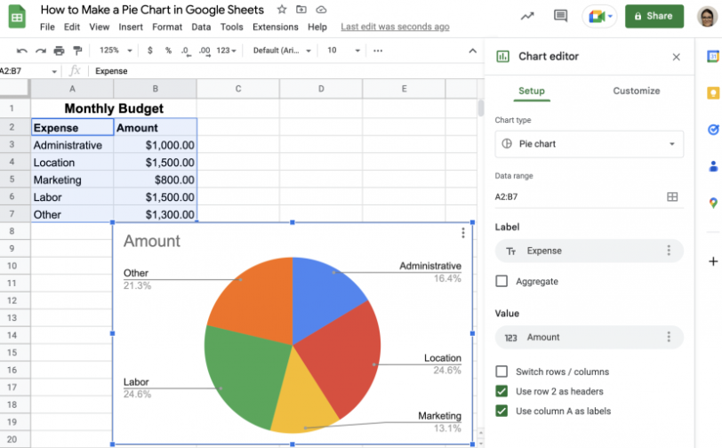
Image Source: productivityspot.com
First things first, let’s get started by opening up Google Sheets and creating a new spreadsheet. Once you have your blank canvas ready, it’s time to input your data. Whether you’re tracking sales numbers, survey results, or any other type of data, pie charts are a great way to showcase your information in a visually appealing format.
Now that you have your data inputted, it’s time to slice it up and create your pie chart. In Google Sheets, creating a pie chart is as easy as selecting your data and clicking on the Insert tab. From there, you can choose the Chart option and select Pie chart from the dropdown menu. Voila! Your pie chart is now ready to be customized.
Image Source: golayer.io
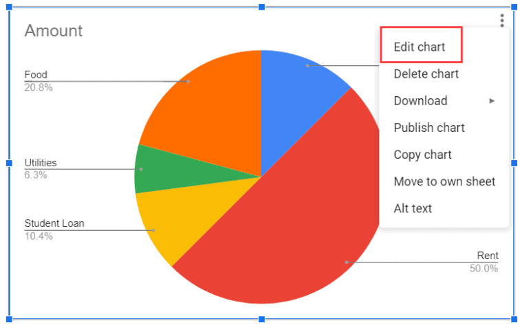
Speaking of customization, let’s whip up a whirlwind of creativity and make your pie chart truly unique. Google Sheets offers a variety of customization options, such as changing the colors, labels, and even the size of your pie chart. You can also add a title and a legend to make your chart more informative and visually appealing.
As you continue to customize your pie chart, keep in mind some chart-topping tips for a perfect finish. Make sure to keep your colors consistent and easy to read, avoid cluttering your chart with too much information, and always double-check your data to ensure accuracy. With these tips in mind, your pie chart is sure to be a showstopper.
In conclusion, creating stunning pie charts in Google Sheets is a fun and creative way to visualize your data. By following this step-by-step guide and incorporating your own unique flair, you’ll be able to impress your colleagues and clients with eye-catching pie charts that make a statement. So what are you waiting for? Let’s get started on your pie chart party today!
Slice it Up: Adding Data to Your Chart
Welcome back to our step-by-step guide to making stunning pie charts in Google Sheets! In our previous article, we got the party started by introducing you to the basics of creating a pie chart. Now, it’s time to slice it up and add some delicious data to your chart.
Adding data to your pie chart is where the magic happens. It’s where you get to showcase your information in a visually appealing and easy-to-understand way. So grab your virtual knife and let’s get slicing!
First things first, open up your Google Sheets and select the data you want to include in your pie chart. This could be anything from sales figures to survey responses to your favorite pie flavors. Once you’ve selected your data, click on the Insert menu at the top of the screen and select Chart.
A new window will pop up, giving you the option to choose the type of chart you want to create. Select Pie chart from the list of options and watch as your data magically transforms into a beautiful pie chart on your screen.
Now, it’s time to customize your chart even further by adding labels and legends. Labels are important for identifying the different slices of your pie chart, while legends provide additional context for your data. To add labels and legends, simply click on the Customize tab in the chart editor and play around with the options until you’re happy with the look of your chart.
But don’t stop there! You can also add colors, adjust the size of your slices, and even explode certain sections of your pie chart to draw attention to specific data points. The possibilities are endless when it comes to customizing your pie chart in Google Sheets.
Once you’ve added all the data you want to your chart, take a step back and admire your handiwork. Your pie chart should now be a visually appealing representation of your data, ready to be shared with colleagues, clients, or friends.
But before you hit that publish button, there are a few more things to consider. Make sure your chart is easy to read and understand by keeping labels clear and concise. Avoid using too many colors or overly complicated designs that could distract from the main message of your chart.
And don’t forget to double-check your data to ensure accuracy. Nothing ruins a stunning pie chart faster than incorrect or outdated information. So take the time to review your data before finalizing your chart.
With your data added and your chart customized to perfection, you’re now ready to slice it up and serve your stunning pie chart to the world. Whether you’re presenting at a board meeting, sharing insights with your team, or simply showing off your data visualization skills, your pie chart is sure to make a lasting impression.
So go ahead, slice it up and add some data to your chart. With a little creativity and a touch of flair, you’ll be well on your way to creating stunning pie charts in Google Sheets that are as delicious to look at as they are informative.
Whip up a Whirlwind: Customizing Your Pie
So you’ve got your data all set and your pie chart is looking pretty good. But why settle for good when you can make it stunning? Customizing your pie chart in Google Sheets is where you can really let your creativity shine. Here are some tips and tricks to help you whip up a whirlwind of a pie chart.
First things first, let’s talk about colors. A pie chart with bland, default colors is like a cake without frosting – it’s just not as fun. Google Sheets gives you the option to customize the colors of each slice of your pie chart. Click on a slice to select it, then right-click and choose Change colors. You can choose from a variety of preset colors, or create your own custom color scheme. Play around with different combinations until you find one that really pops.
Next, let’s talk about labels. Labels are important for helping viewers understand the data in your chart. By default, Google Sheets will display the percentage or value of each slice next to it. But you can customize these labels to make them stand out. Click on a slice to select it, then right-click and choose Edit data labels. You can change the font, size, color, and position of the labels to make them more visually appealing.
Another fun way to customize your pie chart is by adding a title. A title can help give context to your chart and make it more visually appealing. To add a title, click on the chart to select it, then click on the Chart editor button in the toolbar. In the Chart editor panel, click on Customize and then Chart & axis titles. You can add a title for the overall chart, as well as titles for the x and y axes if applicable. Get creative with your titles to make them eye-catching and informative.
If you want to take your customization to the next level, consider adding annotations to your pie chart. Annotations are additional text or shapes that provide extra information about the data in your chart. To add an annotation, click on the chart to select it, then click on the Chart editor button in the toolbar. In the Chart editor panel, click on Annotations and then Add. You can add text or shapes, change the color and size, and position the annotation wherever you like on the chart.
Don’t forget about the overall look and feel of your pie chart. Google Sheets gives you the option to customize the background color, gridlines, and other visual elements of your chart. Click on the chart to select it, then click on the Chart editor button in the toolbar. In the Chart editor panel, you can explore the various customization options available to make your chart look polished and professional.
One final tip for customizing your pie chart is to consider the overall theme or style you want to convey. Are you going for a sleek, modern look? Or maybe a fun, playful vibe? Think about the colors, fonts, and overall design elements that will help you achieve the look you want. Experiment with different customization options until you find the perfect combination that reflects your personal style.
In conclusion, customizing your pie chart in Google Sheets is a fun and creative process that allows you to make your data come to life. By playing around with colors, labels, titles, annotations, and other visual elements, you can create a stunning pie chart that will impress your audience. So go ahead, whip up a whirlwind of a pie chart and show off your design skills!
Chart-topping Tips for a Perfect Finish
When it comes to creating stunning pie charts in Google Sheets, there are a few key tips and tricks that can help you achieve a perfect finish. From choosing the right colors to adding labels and adjusting the chart settings, these chart-topping tips will take your data visualization to the next level.
One of the first things to consider when creating a pie chart is the color scheme. Choosing the right colors can make a big difference in how your chart looks and how easy it is to read. Stick to a simple color palette with contrasting colors to make sure that each slice of the pie stands out. You can also use shades of the same color for a more cohesive look.
Adding labels to your pie chart is another important step in creating a visually appealing chart. Labels can help viewers understand the data more easily and add context to the chart. Make sure to include labels for each slice of the pie, as well as a title for the chart itself. You can also adjust the font size and style to make the labels stand out.
Customizing the appearance of your pie chart is also key to achieving a perfect finish. Google Sheets offers a range of customization options, including adjusting the size of the chart, adding a background color, and changing the chart type. Experiment with different settings to find the look that works best for your data and presentation style.
Another important tip for creating a perfect pie chart is to make sure that your data is accurate and up-to-date. Double-check your data before creating the chart to avoid any errors or inaccuracies. If you need to make changes to the data, you can easily update the chart by editing the source data in Google Sheets.
When it comes to presenting your pie chart, consider the audience and the purpose of the chart. If you are presenting to a professional audience, make sure that the chart is clear, concise, and easy to understand. You can also add annotations or notes to provide additional context for the data.
In addition to these tips, there are a few more advanced techniques that can help you create a truly stunning pie chart. For example, you can use Google Sheets’ interactive features to add tooltips, animation, and interactivity to your chart. This can make the chart more engaging and dynamic, as well as provide additional insights into the data.
Overall, creating a perfect pie chart in Google Sheets is all about attention to detail and experimentation. By following these chart-topping tips and taking the time to customize your chart, you can create a visually appealing and informative data visualization that will impress your audience and help you communicate your message effectively.
how to create pie chart in google sheets


