
Pie Chart Magic: Excel’s Secret Weapon
When it comes to data visualization, pie charts are a powerful tool that can help you make sense of complex information at a glance. And with Excel’s built-in features, creating visually stunning pie charts has never been easier. In this article, we will uncover the secrets behind mastering the art of pie chart creation in Excel.
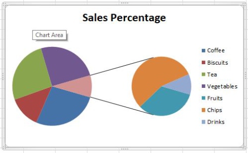
Image Source: geeksforgeeks.org
Excel has long been known for its number-crunching capabilities, but many users overlook its potential for creating beautiful graphics. With just a few clicks, you can transform boring data tables into eye-catching pie charts that will impress your colleagues and clients alike.
The key to creating visually stunning pie charts lies in understanding how to properly format your data within Excel. By organizing your data in a clear and concise manner, you can ensure that your pie chart is both easy to read and visually appealing.
To get started, simply select the data that you would like to represent in your pie chart. This could be anything from sales figures to customer demographics. Once you have selected your data, navigate to the Insert tab at the top of the Excel interface and click on the Pie Chart option.
Excel will then generate a basic pie chart based on your selected data, but the real magic happens when you begin to customize it. By clicking on the various elements of the chart, such as the slices or the legend, you can adjust colors, labels, and other visual elements to make your chart truly unique.
One of the most powerful features of Excel’s pie chart tool is the ability to add data labels. These labels can provide additional context to your chart, making it easier for viewers to understand the data being presented. You can customize the font, size, and position of these labels to ensure that they complement the overall design of your chart.
In addition to data labels, Excel also allows you to add a title and a legend to your pie chart. These elements can help provide further clarity to your visualization and make it more engaging for your audience. By experimenting with different fonts, colors, and layouts, you can create a pie chart that is both informative and visually appealing.
Another trick to mastering pie chart creation in Excel is to leverage the power of formatting options. Excel offers a wide range of customization features, including 3D effects, shadows, and gradients, that can take your pie chart to the next level. By playing around with these options, you can create a chart that is truly unique and eye-catching.
Once you have perfected the design of your pie chart, you can easily share it with others by exporting it to a variety of formats, such as PDF or image files. This makes it simple to include your chart in presentations, reports, or emails, allowing you to communicate your data effectively and impressively.
In conclusion, Excel’s pie chart tool is a secret weapon for anyone looking to create visually stunning graphics with ease. By following the tips and tricks outlined in this article, you can master the art of pie chart creation in Excel and take your data visualization skills to the next level. So why wait? Start creating your own pie charts today and unleash your inner artist with Excel!
Unleash Your Inner Artist with Excel
Do you ever feel like your data reports could use a little more pizzazz? Are you tired of presenting the same old boring charts and graphs to your colleagues or clients? Well, fear not, because Excel is here to help you unleash your inner artist and transform your data into eye-catching graphics that will leave everyone impressed.
Creating visually stunning pie charts in Excel may seem daunting at first, but with a little creativity and some helpful tips, you can master the art in no time. So grab your virtual paintbrush and let’s dive into the world of data visualization!
The first step to creating a visually stunning pie chart in Excel is to choose the right data. Make sure your data is clear, concise, and relevant to the message you want to convey. Remember, the beauty of a pie chart lies in its simplicity, so don’t overcrowd it with too much information.
Next, it’s time to select your chart type. Excel offers a variety of chart options, but for creating a pie chart, you’ll want to choose the Pie Chart option from the Insert menu. Once you’ve selected your data and chart type, it’s time to get creative with colors and formatting.
One of the easiest ways to elevate your pie chart is by customizing the colors. Excel offers a range of color options, but don’t be afraid to mix and match to create a visually appealing color palette. You can also add a splash of creativity by using gradients or patterns to make your chart stand out.
In addition to colors, you can also customize the formatting of your pie chart to make it more visually appealing. Play around with font styles, sizes, and effects to add a touch of personality to your chart. You can also experiment with chart elements such as labels, legends, and data points to make your chart more informative and engaging.
Another way to unleash your inner artist with Excel is by adding a touch of interactivity to your pie chart. Excel allows you to add interactive features such as tooltips, hyperlinks, and animations to make your chart more engaging and dynamic. These interactive elements can help you tell a story with your data and keep your audience engaged.
Once you’ve customized your pie chart to perfection, it’s time to present your masterpiece. Excel offers a range of options for sharing your charts, including printing, emailing, or embedding them in a presentation. You can also save your chart as an image or PDF file to easily share it with others.
In conclusion, creating visually stunning pie charts in Excel is a fun and creative process that can help you transform your data into eye-catching graphics. By choosing the right data, customizing colors and formatting, adding interactivity, and presenting your chart with flair, you can unleash your inner artist and impress your audience with your data visualization skills. So go ahead, embrace your creative side and start creating pie charts that are as beautiful as they are informative.
Transform Data into Eye-catching Graphics
Do you often find yourself staring at rows and columns of data in Excel, wondering How to Make it more visually appealing? Do you wish there was a way to transform that data into eye-catching graphics that are not only informative but also aesthetically pleasing? Well, look no further because Excel has the tools you need to turn your boring data into stunning visuals that will impress your colleagues and clients.
Creating visually appealing graphics in Excel doesn’t have to be a daunting task. With a few simple steps, you can easily transform your data into eye-catching pie charts that will grab the attention of anyone who sees them. Whether you’re presenting sales figures, budget breakdowns, or survey results, pie charts are a great way to visually represent your data in a way that is easy to understand and visually appealing.
The key to creating visually stunning pie charts in Excel is to first organize your data in a way that makes sense. Make sure your data is clean and easy to read, with clear labels and categories. Once your data is organized, select the data you want to include in your pie chart and click on the Insert tab at the top of the Excel window.
From the Insert tab, select the Pie Chart option to see a variety of pie chart options to choose from. You can select a basic pie chart, a 3D pie chart, or even a pie chart with exploded slices to add extra visual interest. Once you’ve selected the type of pie chart you want to create, Excel will generate a basic pie chart based on your selected data.
But why stop at a basic pie chart when you can take it to the next level with a few simple customizations? Excel gives you the ability to customize every aspect of your pie chart, from the colors of the slices to the labels and legends. You can even add data labels to your pie chart to make it easier for your audience to understand the data you’re presenting.
To customize your pie chart, simply right-click on any element of the chart and select the Format option. From here, you can change the colors of the slices, adjust the size and position of the labels, and even add a title to your chart. You can also change the chart type from a pie chart to a doughnut chart or a bar chart, depending on your preferences.
With a few simple customizations, you can transform your basic pie chart into a visually stunning graphic that will impress everyone who sees it. And the best part is, you don’t need to be a graphic designer or Excel expert to create these eye-catching visuals. With just a little bit of creativity and some basic Excel skills, you can turn your boring data into stunning graphics that will make your presentations stand out.
So why settle for boring, uninspired data presentations when you can easily transform your data into eye-catching graphics with Excel? Master the art of creating visually stunning pie charts in Excel with ease and watch as your colleagues and clients are blown away by your newfound graphic design skills. Excel may be known for its number-crunching abilities, but with a little creativity, it can also be a powerful tool for creating beautiful and informative graphics that will take your presentations to the next level.
Easy Steps to Pie Chart Perfection
Are you ready to master the art of creating visually stunning pie charts in Excel with ease? Look no further, because we’ve got the easy steps you need to achieve pie chart perfection in no time!
Pie charts are a powerful tool for visualizing data and making it easy to understand at a glance. With just a few simple steps, you can transform boring numbers into eye-catching graphics that will impress your colleagues and clients.
Step 1: Organize Your Data
Before you can create a pie chart, you need to make sure your data is organized properly. In Excel, this means putting your data into columns or rows with clear labels for each category. This will make it easier to create a pie chart that accurately represents your data.
Step 2: Select Your Data
Once your data is organized, it’s time to select the data you want to include in your pie chart. Simply click and drag to highlight the data you want to use, making sure to include both the category labels and the corresponding values.
Step 3: Insert Your Pie Chart
With your data selected, it’s time to insert your pie chart. In Excel, this is as simple as clicking on the Insert tab and selecting Pie Chart from the chart options. Choose the style of pie chart you want to use, whether it’s a traditional pie chart or a 3D pie chart, and watch as Excel creates your chart for you.
Step 4: Customize Your Pie Chart
Now that you have your pie chart, it’s time to customize it to make it visually stunning. You can change the colors of the chart slices, add labels and titles, and even adjust the size and position of the chart within your Excel sheet. Play around with different options until you find the perfect look for your pie chart.
Step 5: Add Data Labels
To make your pie chart even more informative, consider adding data labels to each slice. This will make it easy for viewers to see the exact values represented by each part of the chart, making your data more accessible and understandable.
Step 6: Explode Your Chart
For added visual impact, you can explode your pie chart by pulling out one or more slices from the rest of the chart. This can help draw attention to specific data points or categories, making your chart even more engaging and informative.
Step 7: Format Your Chart
Finally, don’t forget to format your pie chart to make it look polished and professional. You can adjust the font style and size, add a legend to explain the different colors in your chart, and even add a border or shadow to make your chart stand out.
With these easy steps, you can master the art of creating visually stunning pie charts in Excel with ease. Impress your colleagues and clients with beautiful, informative charts that make your data come to life. So go ahead, unleash your inner artist and start creating pie chart perfection today!
how to create pie chart in pie chart excel


